Python Code for Mapping Data Flow Users: Part 1 - Multiple Inputs
Why Learn Python
Microsoft has published a how-to guide for Dataflows Gen2. In it they maintain:
Microsoft Fabric’s Data Factory experience provides an intuitive and user-friendly interface using Power Query Online that can help you streamline your data transformation workflows when authoring Dataflow Gen2. If you’re a developer with a background in Azure Data Factory and Mapping Data Flows, you’ll find this guide helpful in mapping your existing Mapping Data Flow transformations to the Dataflow Gen2 Power Query user interface.
So, I have put together this and subsequent posts to demonstrate how the functionality can be achieved from Notebooks using Python as would be used in Mapping Data flow.

A couple of specific examples:

These Transforms allow for data from multiple sources to be joined, merged and identified.

For the join example, I will concentrate on the INNER JOIN but as we look at other transformations we consider other joins.

In this example, two separate streams are created using a filter on department_id. Clauses for filters can be more complex than this and the use of multiple conditions. The syntax will use && for AND while || is used for OR. This should be familiar for those experienced with Mapping Data flow expression language. For more detail see here: pyspark.sql.DataFrame.filter — PySpark 3.5.0 documentation (apache.org)


Loading Data
The first challenge will be to create a source. Notebooks are more than capable of loading data from many sources. 


Considering the above sources the notion of an integration dataset is probably not applicable but we can easily collect data from specific file types and from lake databases (workspace DB).
Loading from a file.
Loading from files within a lake storage is straightforward and the options required are well documented.
Loading a csv file:
sourceData = spark.read.load(source_file,format = 'csv',delimiter = '|',header=True)display(sourceData.limit(10))
In this example, the generic Load method is used with some options specified. I have used source_file, a variable determining the specific location within the data set.
- The format stipulates a CSV file and could as easily specify JSON or Parquet. An alternative method spark.read.csv would work similarly well. Again, methods exist for other file types.
- I have specified a pipe delimiter.
- I have specified that the file contains a header row.
In this approach the options are all specified inside the method [load]. This is valid alternative but in this case the options are explicitly called out with the option keyword.
Loading from a Table
As an analogue for using the Workspace DB source, loading data from lake databases is incredibly simple. In this example, database and table are both parameters.
sqlString = f'SELECT * FROM {database}.{table}'dataSourceToo = spark.sql(sqlString)display(sourceData.limit(10))
Example data
It is also possible to specify data in code. In subsequent examples I will use this data for demonstration purposes.
employee = (spark.createDataFrame([(0, "Jason Arancione", 0, [100,750,250]),(1, "Giacomo Marrone", 2, [500,250,100]),(2, "Eva Prugna", 0, [250, 1000]),(3, "Ambra Sentito", 1, [250, 1000]),(4, "Graham Verde",5,[250, 1000,500,750])]).toDF("id","name","department_id","skill_set"))department = (spark.createDataFrame([(0,"Data Engineering","DER","Data Engineering Business Systems"),(1,"Data Analytics","DER","Reporting and Business Itelligence"),(2,"Applications","AWP","Business Applications and Product Dev"),(3,"Web","AWP","E-Commerce and Applications"),]).toDF("id","department_name","directorate","business_unit"))skill = (spark.createDataFrame([(1000,"html" ),(750,"SQL" ),(500,"c#" ),(250,"Java" ),(100,"python"),]).toDF("id", "skill"))
Multiple Input Transforms.

These Transforms allow for data from multiple sources to be joined, merged and identified.
Join
The simplest of these is the JOIN transformation. This operates much as a SQL join would. Dataframe joins are relatively simple and most of the applications that follow use spark.sql.Dataframe.join methods.

In all joins I will use the following Join expression.
joinExpression = employee["department_id"] == department["id"]
The join method is relatively straightforward after that.
joinDF is a dataframe that is equal to employee INNER JOIN department ON departement_id = id
The Join function is a method of dataframe requiring the second table and the expression for joining. This can be defined at the time of the join or, in my case, before the join operation. The final, optional, parameter is the type of join. Omitting this will default to an inner join.
joinDF = employee.join(department, joinExpression,'inner')
Conditional Split
The conditional split transformation is designed to route data to different streams based on a filter or match condition. There are two options to split the data:
- First Matching Condition
- All Matching Conditions

When writing code to simulate this the simplest to describe would be the second option, it is my experience that the first option is likely the more common. Thought and care should be taken when splitting data to enforce the behaviour required and more complex conditions might be required to ensure the proper separation of data. The default - where no condition is met does not naturally occur and code would be needed to satisfy this.
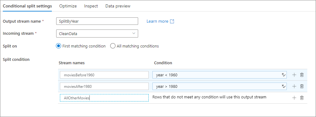 |
| From Microsoft Learn: Split conditions. |
dataEngineers = employee.filter(employee['department_id'] == 0)otherPeople = employee.filter(employee['department_id'] != 0)
Union
Once we have separated the data we can rejoin the data if we wish.

The behaviour of a Union has two options either Union by Name or by Position. These can both be replicated and the Pyspark documentation is very expansive on the behaviour.
- pyspark.sql.DataFrame.union is the same as Union by position.
- pyspark.sql.DataFrame.unionByName is (obviously) Union by
The following examples are instructive for syntax but as above we know these have the same schema so will essentially deliver the same result. For varying schema, unionByName offers the ability to match common columns and populate NULL values where columns for either source are unique. This behaviour is the same as we see with Data Flow Transformations.
union = dataEngineers.union(otherPeople)

display(union)

unionbyname = dataEnginers.unionByName(otherpeople)

display(unionbyname)
Exists
The Exists transformation checks whether your data exists in another source or stream. We have two options when we use the transformation.
- Does it exist
- Does it not exist

Both options rely on the Join operation. Remember for these examples we use the join Expression specified above. This could be more complex if necessary with multiple clauses.
exists
For the exists option we use the Semi Join, this join doesn't include any values from the Left DataFrame. It compares to see if value exists in second DataFrame. If the value does exist, those rows will be kept in the result, even if there are duplicate keys in the left DataFrame.
- semi
- leftsemi
- left_semi
Each version of the syntax produces the same result.
display(employee.join(department, joinExpression, 'semi'))
does not exist
The opposite of the Semi Join is the Anti Join. In SQL terms this is akin to the NOT IN clause.
All syntax returns the same result.
- anti
- leftanti
- left_anti
display(employee.join(department, joinExpression, 'anti'))
Lookup
Lookup is described as "Reference data from another source". In reality this operates like a Left Join.
- left
- leftouter
- left_outer

Each syntax returns the same result.
display(employee.join(department, joinExpression, 'left'))
Conclusion
Using Pyspark it is very simple to achieve similar results as those of Mapping Data Flow for multiple sources. Some of the features require some additional thought but this thought process should be applied to Mapping Data Flow too.


Comments
Post a Comment